This tutorial will walk through how to leverage the
tidyCDISC app’s Table Generator tab. Let’s walk through
creating simple summary statistics, among other things. If you haven’t
already, import your studies data. For this tutorial, we’ll be using the
five CDISC Pilot data files: An ADSL, ADVS,
ADLBC, ADAE, and the ADTTE.
Building an example table from scratch
The Table Generator tab is divided in two: the area to the left is the drag-and-drop interface used to build tables, and on the right is the real-time table output.
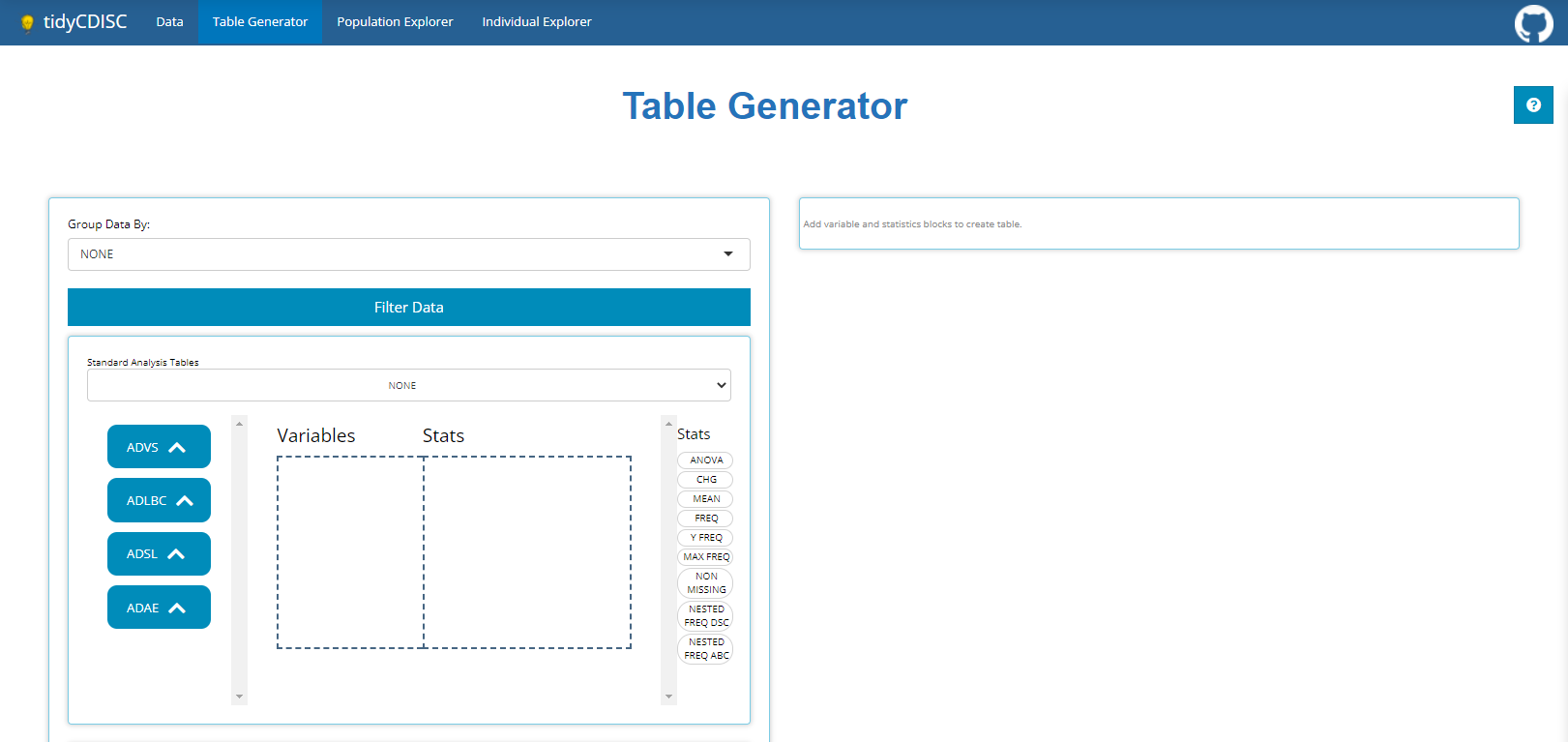
Any uploaded data sets will appear on the left-hand side as “bins”.
“Bins” are just containers, showcasing the usable contents from a data
source, when expanded. The ADSL & ADAE
bins include the names of all their variables, while any
BDS data sets, like the ADVS &
ADLBC bins include a list of all the PARAMCD
values. TTE class data sources are currently not supported
in the table generator.
On the right-hand side, there are a list of “Stats”, such as
ANOVA, CHG, MEAN, and
FREQ to name a few. We call these “STAT Blocks”. And
finally, in the middle of it all is the “drop zone”.
In order to build a table, we need only drag a variable block to the “Variable” drop zone and match it up with an applicable stat block by dragging it in the “Stats” drop zone, demonstrated in the following example.
Age Summary Statistics
Below, we drag the AGE block from the ADSL
and drag the MEAN block from the list of Stats to calculate
summary statistics on patient AGE within the trial.
PARAMCD Summary Statistics
Similarly, we can drag in DIABP from the
ADVS and use the MEAN block to calculate
summary statistics on parameters. However, because DIABP
came from a BDS class data source, we need to select the
desired AVISIT to calculate summary statistics for the
desired time point.
Add FREQ stat to categorical variable block, re-shuffle, and delete output
Now let’s assume we forgot to add some frequency statistics for our
studies age groups. In fact, we really prefer it over the quantitative
statistics previously calculated on the AGE variable. It’s
no problem! We simply go back to our ADSL bin, select &
move the AGEGRP1 variable to the “drop zone” and pair it
with a FREQ stat block. Recently added blocks are always
added to the bottom of the list, but that’s no worry, once added, you
can shuffle the blocks around to present the output in the most logical
manner. To remove an undesired output, just click the X on
the right-hand side of each variable & corresponding stat block.
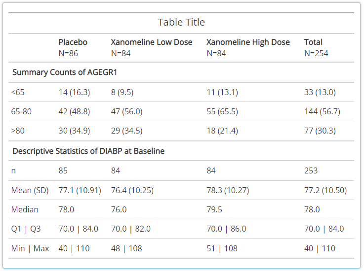
Group by another Variable
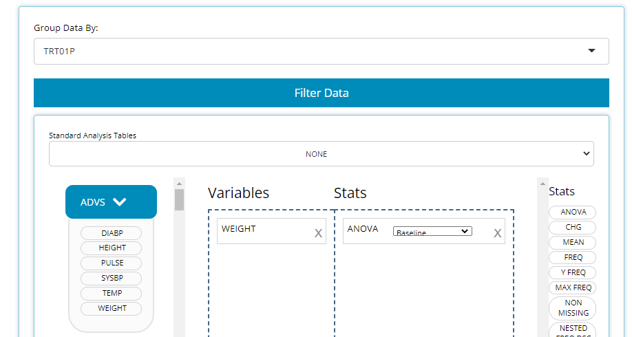
We can use the ‘Group By’ drop-down list to
calculate our table’s statistics across levels of a categorical
variable. For example, When we select TRT01P, the a single
column of statistics is broken down by all the planned treatment
groups.
Here is the resulting table:
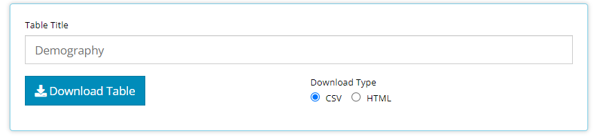
Title and download table output
Now that we’ve created a simple table, it’s time to name and download it for saving/ sharing. Below, we insert our table title and download as CSV. Currently, the app supports RTF, CSV, and HTML output formats, but PDF is coming soon!
That’s it for our example workflow when building tables from scratch. However, the table generator offers many more features, including filtering, other statistical blocks, recipes for standard analysis (STAN) tables, more export file types for output, exported R code to reproduce the table, and in-app guided help. Those topics are expanded on below!
Other Stat blocks
Please use this resource as a guide when determining how to summarize your data. It’s important to note that new statistical blocks are in development, so if they are not listed below, you can hover over any of the stat blocks in the app and text will appear for a “quick reference” description. The stat blocks we showcased in the demo above include the following:
MEAN:Eight summary statistics are displayed. These include n, mean, standard deviation, median, Q1, Q3, Min, and Max.FREQ:Counts and percentages are displaced for all variable values that exist. Note this does not count subjects like the frequencies described below. If you’d like to count subjects, seeNESTED FREQ DSCORNESTED FREQ ABC.
The other statistical blocks not showcased in the demo are:
-
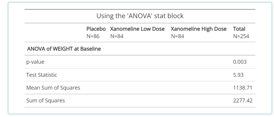
ANOVA:this block can be used in conjunction with the grouping variable drop down selection to determine if means differ across groups.
-
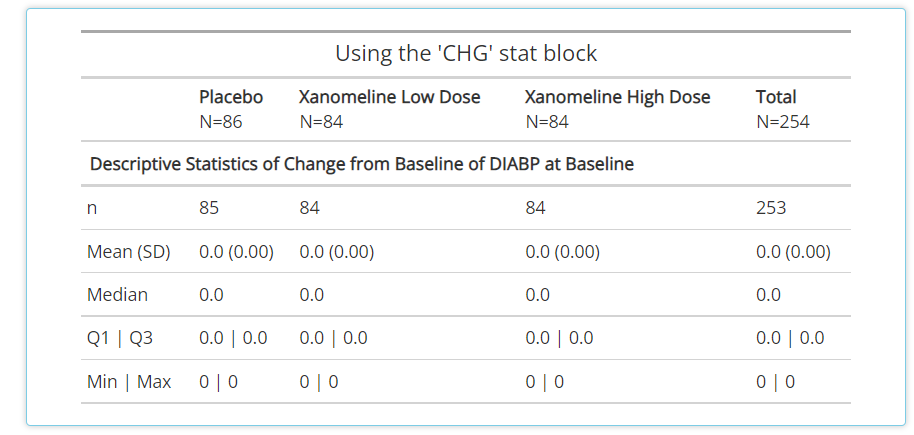
CHG:like the mean block, this also calculates basic summary statistics but uses the change from baseline value rather thanAVAL
-
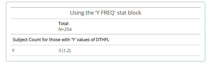
Y FREQ:Only applies to flag variables (ending in ‘FL’, likeDTHFL) that contain ‘Y’ values. The output will include a subject count and percentage for only the ‘Y’ values.
-
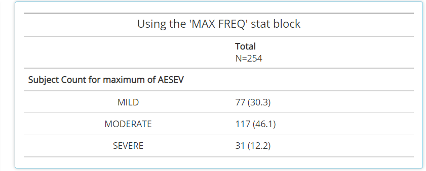
MAX FREQ:This statistic only applies to variables (VAR) that have a “N” (VARN) counterpart. It’s useful for variables likeAESEVwhen subjects should only be counted one time at their max VARN value. So, when paired withAESEVorAESEVN, the frequencies will reflect maximum severity of an adverse event during the trial.
-
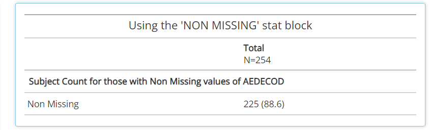
NON MISSING:A handy statistic that counts subjects who have non-missing values for a given variable. As such, it can help provide a high level measure of how many subjects had some value, as seen below withAEDECOD
-
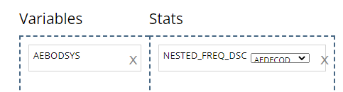
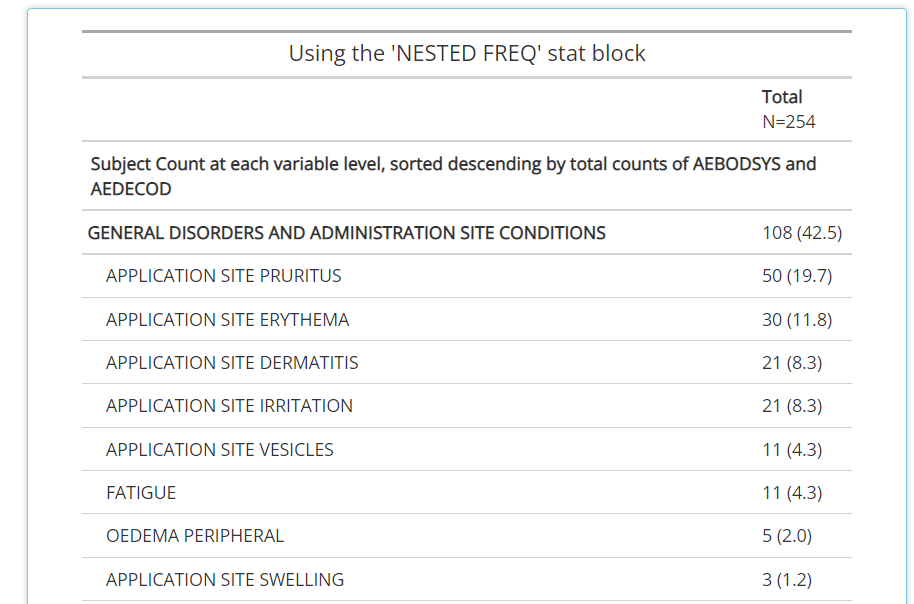
NESTED FREQ DSC:Notice when using this stat block, you’ll need to choose a variable to “nest” inside the values / levels of another. Without the nested variable selected (ieNONEis selected), the subject counts and percentages are displayed in descending order. Place the high level variable (likeAEBODSYS) on the left hand side and select the more granular variable to be “nested” inside of it, likeAEDECOD. Then the output will show all theAEDECODvalues that exist within eachAEBODSYS, all sorted descending.
-
NESTED FREQ ABC:provides the same functionality asNESTED FREQ DSC, but organizes the variables and it’s values in alphabetical order!
Filtering data in the table generator
There is an entire guide called “04
Filtering” dedicated to filtering in the tidyCDISC
application. Please reference that article as the ultimate filtering
resource, but just note that when filtering occurs on the Table
Generator tab, those filters permeate all data sets on
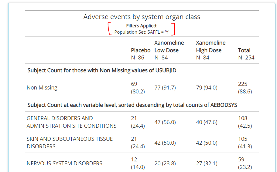
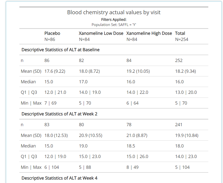
the tab and will be reflected in the table output as seen below. Also
note that some mandatory filters will be applied automatically when
‘standard analysis’ tables are selected so be aware of the filtering
caption displayed beneath the table title (red brackets added for
attention). Ultimately, it is the users responsibility to make sure the
correct data filters are applied for their table output!
Standard Analysis Tables
There are a set of tables / listings that users need to build frequently, due to their common inclusion in submission filings to regulatory authorities. As such, the Table Generator (at the time this guide was authored) contains the following ‘recipes’ for commonly used tables:
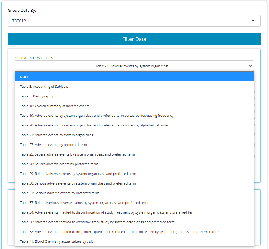
When data needed to produce certain outputs aren’t present, the list
of available tables in this drop down will change. For example, if an
ADAE is not uploaded, then all the AE tables will disappear
from the above list.
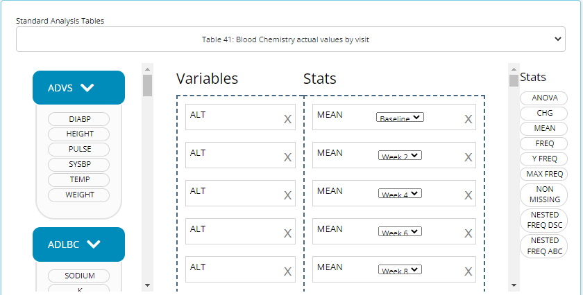
When one of these tables is selected, the table generator simply
compiles the needed variable and stat blocks in the correct order to
generate the desired output. This can be particularly useful for tables
like #41 “Blood Chemistry actual values by visit” since it would be
cumbersome to manually drag in a MEAN block for each week
and each blood chemistry parameter, as there can be many. See snapshot
of this automation below:
Export output file types
As displayed in an earlier demo, you can export table output to an
RTF, CSV, or HTML file. In a future release of tidyCDISC,
you’ll be able to prepare a PDF version of your output. In the meantime,
you can create a PDF using a temporary work-around: first export as
HTML, then download page as a PDF.
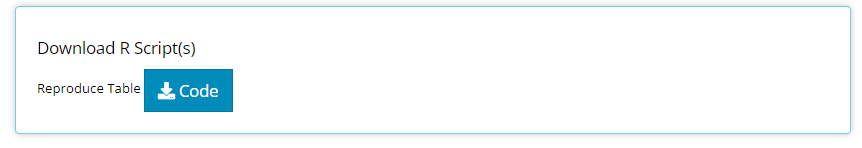
Export R code to reproduce table outside of app
As previously mentioned, one can reproduce any table created inside the app in an R script by downloading code using this button:
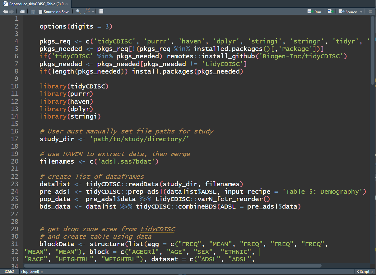
Upon doing so, the R script will download to your browser and when
opened in R Studio, should look something like the below image. The R
script will help you install any packages needed for the analysis,
including the tidyCDISC package. If you used the CDISC
Pilot data, no code modification is needed to reproduce the output since
that data is pre-loaded into the tidyCDISC package.
However, if you uploaded your data from a different source, you’ll need
to enter the file path to your study directory’s data as a string, as
seen on line 17. Note: 'path/to/study/directory/' is just a
placeholder until you enter your own string. If you are unsure of how to
format your string, just run choose.dir() in your R console
if running on Windows.
After reading in the data, the R script will recall the variable and stat blocks previously dropped into the “drop zone” to recreate the output using the exact same process as performed in the app. From there, an R data.frame and html rendering of your table is prepared for saving or further analysis.
Need help?
Throughout all the tabs in the application, there are these little buttons (usually in the top right-hand corners) with question marks on them:

When clicked, they launch a real-time guide that walks the user through the major components of the currently visible screen/ tab, providing context and suggested workflow. However, if the in-app guide doesn’t address your needs, consult the online documentation (that you’re reading now) for the most thorough user guide. If all else fails, send the developers a message with your question or request!